Building a quantum circuit simulator

Introduction

Over the past few weeks, I've been exploring quantum computing by building QNano, a lightweight quantum circuit simulator written in Rust. It simulates two qubits which creates a surprisingly rich playground for quantum algorithms. QNano provides an easy assembly-like scripting language that can be used for rapid prototyping and experimentation with quantum gates.

You can find the full project on GitHub.

This blog post will focus on the simulation of qubits and therefore only provide a basic introduction to the mathematics behind qubits and quantum gates. I recommend reading Quantum computing for the very curious which provides an excellent introduction to the mathematics behind quantum computing.

What are qubits?

In classical computing, a bit is either $0$ or $1$. It's simple and deterministic. However, in quantum computing, a qubit can be $0$ and $1$ at the same time, existing in what physicists call superposition. Mathematically, we write a qubit's state as:

$$ |\psi\rangle = \alpha|0\rangle + \beta|1\rangle $$

Here, $\alpha$ and $\beta$ are complex numbers called probability amplitudes. The key constraint is that they must satisfy:

$$ |\alpha|^2 + |\beta|^2 = 1 $$

This ensures that when we measure the qubit, the probabilities add up to 100%. We'll find it in state $|0\rangle$ with probability $|\alpha|^2$ and in state $|1\rangle$ with probability $|\beta|^2$.

Why vectors?

One might wonder why we talk about qubits as vectors. The reason is that quantum states mathematically live in a vector space. The states $|0\rangle$ and $|1\rangle$ are what we call the computational basis states, and they form an orthonormal basis for this space. In concrete terms, we can write these basis states as column vectors:

$$ |0\rangle = \begin{bmatrix} \ 1 \ \\[0.3em] \ 0 \ \end{bmatrix} \quad |1\rangle = \begin{bmatrix} \ 0 \ \\[0.3em] \ 1 \ \end{bmatrix} $$

Any qubit state is then a superposition (linear combination) of these basis vectors:

$$ |\psi\rangle = \alpha|0\rangle + \beta|1\rangle = \alpha\begin{bmatrix} \ 1 \ \\[0.3em] \ 0 \ \end{bmatrix} + \beta\begin{bmatrix} \ 0 \ \\[0.3em] \ 1 \ \end{bmatrix} = \begin{bmatrix} \ \alpha \ \\[0.3em] \ \beta \ \end{bmatrix} $$

This vector representation is crucial because quantum gates are represented as matrices that multiply these state vectors. When we apply a gate to a qubit, we're performing matrix multiplication to transform the state vector.

The computational basis is special because these are the states we can actually measure. When you measure a qubit, it "collapses" to either $|0\rangle$ or $|1\rangle$. You can never measure a qubit and get $0.7$ or some value in between. The probabilities $|\alpha|^2$ and $|\beta|^2$ tell us the likelihood of each outcome, but the measurement itself is always discrete.

Two qubits

For two qubits, the combined system exists in a superposition of four basis states:

$$ |\psi\rangle = c_1|00\rangle + c_2|01\rangle + c_3|10\rangle + c_4|11\rangle $$

Each basis state corresponds to a classical configuration:

• $|00\rangle$ means both qubits are 0
• $|01\rangle$ means qubit 0 is 0 and qubit 1 is 1
• $|10\rangle$ means qubit 0 is 1 and qubit 1 is 0
• $|11\rangle$ means both qubits are 1

To simulate this two-qubit system classically, we need to track all four complex amplitudes that describe the state vector. In QNano, this is represented as an array:

struct QuantumCircuit {
    state: [Complex64; 4], // |00⟩, |01⟩, |10⟩, |11⟩
}

impl QuantumCircuit {
    fn new() -> Self {
        Self {
            state: [
                Complex64::new(1.0, 0.0),  // |00⟩ amplitude
                Complex64::new(0.0, 0.0),  // |01⟩ amplitude
                Complex64::new(0.0, 0.0),  // |10⟩ amplitude
                Complex64::new(0.0, 0.0),  // |11⟩ amplitude
            ],
        }
    }
}

We initialize the state to $|00\rangle$ by setting the first amplitude to 1 and the rest to 0. This is the usual starting point.

Notice the difference between the quantum system and simulating it classically. A quantum computer only needs two physical qubits to represent this state, but our classical simulation must explicitly store all four amplitudes.

This scaling continues: for $n$ qubits, we need to track $2^n$ amplitudes. At 10 qubits, that's 1,024 amplitudes. At 30 qubits, it's over a billion. This exponential growth is why classical simulation of quantum systems becomes impractical beyond a few dozen qubits. Quantum computers are able to simulate these state spaces directly.

Quantum gates

In quantum computing, we have quantum gates that perform unitary transformations on qubits. These gates manipulate the probability amplitudes while preserving the total probability.

The X Gate

The simplest gate is the X gate, which is the quantum equivalent of a classical NOT gate. It flips $|0\rangle$ to $|1\rangle$ and vice versa:

$$ X|0\rangle = |1\rangle \quad \quad X|1\rangle = |0\rangle $$

In QNano, this is implemented by swapping the appropriate amplitudes:

fn apply_x(&mut self, q: usize) {
    match q {
        0 => {
            self.state.swap(0, 2);  // swap |00⟩ ↔ |10⟩
            self.state.swap(1, 3);  // swap |01⟩ ↔ |11⟩
        },
        1 => {
            self.state.swap(0, 1);  // swap |00⟩ ↔ |01⟩
            self.state.swap(2, 3);  // swap |10⟩ ↔ |11⟩
        },
        _ => println!("Error: qnano only supports qubits 0 and 1!"),
    }
}

The Hadamard Gate

The Hadamard gate is more interesting. It puts a qubit into an equal superposition of the basis states $|0\rangle$ and $|1\rangle$. Mathematically, the Hadamard gate can be represented as the following matrix:

$$ H = \frac{1}{\sqrt{2}}\begin{bmatrix} \ 1 & 1 \ \\[0.3em] \ 1 & -1 \ \end{bmatrix} $$

Instead of simply flipping states, it transforms the basis states. After applying Hadamard, both amplitudes become non-zero:

$$ H|0\rangle = \frac{1}{\sqrt{2}}(|0\rangle + |1\rangle) $$

$$ H|1\rangle = \frac{1}{\sqrt{2}}(|0\rangle - |1\rangle) $$

People often say the Hadamard Gate "creates superposition" which is worth clarifying. Mathematically, we saw that any qubit state can be written as $|\psi\rangle = \alpha|0\rangle + \beta|1\rangle$, which we call a superposition of the basis states. But when a qubit is in state $|0\rangle$, we have $\alpha = 1$ and $\beta = 0$. This is a trivial case, since the qubit is definitively in $|0\rangle$ and measuring it gives 0 with 100% probability.

In the case of applying the Hadamard Gate, the qubit has genuine quantum uncertainty. Measuring it gives 0 or 1, each with 50% probability. When we say Hadamard creates superposition, we mean it transforms a definite, classical-like state into one with multiple non-zero amplitudes, a state that exhibits probabilistic behavior when measured.

In QNano, applying Hadamard to qubit 0 means transforming pairs of amplitudes:

fn apply_h(&mut self, q: usize) {
    let s = 1.0 / 2.0_f64.sqrt();

    match q {
        0 => {
            // Pair 1: |00⟩ and |10⟩
            let a = self.state[0];
            let b = self.state[2];
            self.state[0] = (a + b) * s;
            self.state[2] = (a - b) * s;

            // Pair 2: |01⟩ and |11⟩
            let c = self.state[1];
            let d = self.state[3];
            self.state[1] = (c + d) * s;
            self.state[3] = (c - d) * s;
        },
        // ... qubit 1 case
    }
}

Other gates in QNano

QNano also supports:

• Z gate: Flips the phase of $|1\rangle$, mapping $|1\rangle \to -|1\rangle$
• S gate: Applies a 90° phase rotation to $|1\rangle$
• T gate: Applies a 45° phase rotation to $|1\rangle$
• CX gate: Flips the target qubit if the control qubit is $|1\rangle$
• CZ gate: Flips phase if both qubits are $|1\rangle$

These gates form a universal gate set, meaning they can approximate any quantum computation on two qubits.

The QNano scripting language

To make experimenting with quantum circuits easy, QNano uses a simple assembly-style scripting language. Files use the .qnano extension with one instruction per line:

h 0
x 1
cx 0 1

The parser is straightforward, just splitting lines into tokens and matching against gate names:

fn parse_program(contents: &str) -> Vec<Gate> {
    let mut instructions: Vec<Gate> = Vec::new();

    for line in contents.lines() {
        let tokens: Vec<&str> = line.split_whitespace().collect();
        if tokens.is_empty() { 
            continue; 
        }

        match tokens[0] {
            "h" => instructions.push(Gate::H(tokens[1].parse().unwrap())),
            "x" => instructions.push(Gate::X(tokens[1].parse().unwrap())),
            "z" => instructions.push(Gate::Z(tokens[1].parse().unwrap())),
            "s" => instructions.push(Gate::S(tokens[1].parse().unwrap())),
            "t" => instructions.push(Gate::T(tokens[1].parse().unwrap())),
            "cx" => instructions.push(Gate::CX(
                tokens[1].parse().unwrap(), 
                tokens[2].parse().unwrap()
            )),
            "cz" => instructions.push(Gate::CZ(tokens[1].parse().unwrap())),
            _ => print!("Unknown gate: {}", tokens[0]),
        }
    }

    return instructions;
}

You can then run these quantum gate instructions:

qnano your_circuit.qnano

The output shows the final state vector with complex amplitudes for all four basis states.

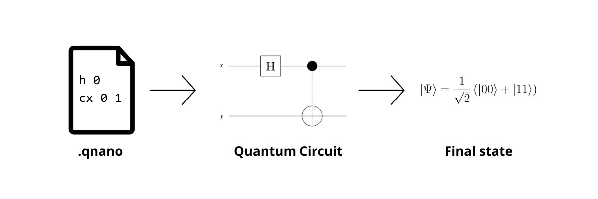
Simulating Bell state

Now it gets exciting! Using these tools we can simulate one of the most famous quantum states, namely the Bell state. It's the simplest example of quantum entanglement. Here's how you create it in QNano:

h 0
cx 0 1

Let's trace through what happens mathematically and then see why these qubits are now entangled.

Step 1: Initial state

We start with both qubits in $|0\rangle$:

$$ |\psi_0\rangle = |00\rangle = \begin{bmatrix} \ 1 \ \\[0.3em] \ 0 \ \\[0.3em] \ 0 \ \\[0.3em] \ 0 \ \end{bmatrix} $$

In QNano's output:

|00>: 1.00+0.00i
|01>: 0.00+0.00i
|10>: 0.00+0.00i
|11>: 0.00+0.00i

Step 2: Apply Hadamard

Next we apply the Hadamard gate to qubit 0. The Hadamard gate puts qubit 0 into superposition:

$$ |\psi_1\rangle = \frac{1}{\sqrt{2}}(|00\rangle + |10\rangle) $$

If we measured qubit 0 now, we'd get 0 or 1 with equal probability.

Step 3: Apply CX

We apply the CX with control = 0 and target = 1. The CX flips qubit 1 whenever qubit 0 is $|1\rangle$. In the $|00\rangle$ component, qubit 0 is 0, so nothing happens. In the $|10\rangle$ component, qubit 0 is 1, so qubit 1 gets flipped to 1:

$$ |\psi_2\rangle = \frac{1}{\sqrt{2}}(|00\rangle + |11\rangle) $$

This is a Bell state. Running QNano gives:

|00>: 0.71+0.00i
|01>: 0.00+0.00i
|10>: 0.00+0.00i
|11>: 0.71+0.00i

The only non-zero amplitudes are for $|00\rangle$ and $|11\rangle$. Why is this interesting?

Notice how before measurement, both qubits are individually in superposition. Each has a 50% chance of being 0 or 1. But their outcomes are not independent. The moment you measure one qubit, you instantly know the other. This is because the states $|01\rangle$ and $|10\rangle$ have zero amplitude, meaning they can never occur. If you measure qubit 0 and get 0, then you also know qubit 1 is definitely 0. Get 1? Qubit 1 is definitely 1.

What makes this strange is that this correlation exists even though neither qubit has a definite value until measured. It's not like a pair of gloves where one is always left and one is always right. With entangled qubits, there's no hidden information. The qubits genuinely don't have definite values until observation, yet they somehow always agree.

The entanglement is also instantaneous. If you had two entangled qubits at opposite ends of the galaxy, measuring one would immediately tell you the value of the other. Einstein called this "spooky action at a distance" and believed it meant quantum mechanics was incomplete. Decades of experiments have confirmed that the correlations are real, but we still don't have a satisfying intuition for how it works.

What I learned from this project

I recently started learning Rust and this was an excellent project to get more familiar with the syntax. Having just finished a course in Quantum Technology, being able to put that knowledge into code was also a great way to solidify the learnings.

Here are two things I learned that stood out:

• Rust's error messages are excellent. As a beginner, I got a lot of help from the Rust compiler. When something went wrong, the compiler pointed to the exact line, explained the problem, and often suggested a fix. This made learning the language much more enjoyable.

• Two qubits is enough to learn the basics. Quantum computing may seem very abstract at first glance, but the truth is that you don't have to understand all of quantum mechanics to understand what is going on. You can do surprisingly much using only two qubits. As shown above, both superposition and entanglement are possible to simulate using only two qubits.

Try it yourself

You can find the full project on GitHub. I would be super happy if you give it a star! You can get started using QNano by installing it:

cargo install --git https://github.com/Cqsi/qnano

Then create a .qnano file and run:

qnano your_circuit.qnano

See if you can create other Bell states or more complex entangled states!

Casimir Rönnlöf, January 2026